# ==============================================================================
# 无治疗病例分析(含IPTW权重)- Jupyter Notebook专用R代码(最终无报错版)
# 功能:数据读取→无治疗病例筛选→描述性统计→Bootstrap分析→IPTW权重→可视化→结果导出
# 适配环境:Jupyter Notebook + R 4.0+(Mac/Windows/Linux通用)
# ==============================================================================
# ------------------------------------------------------------------------------
# 1. 环境配置与包加载(含所有依赖包)
# ------------------------------------------------------------------------------
# 清除环境变量
rm(list = ls())
# 安装必要包(首次运行时取消注释执行,仅需一次)
# install.packages(c(
# "readxl", "dplyr", "tidyr", "ggplot2", "grid", "gridExtra", "boot",
# "Matching", "caret", "broom", "knitr", "kableExtra", "openxlsx",
# "scales", "stringr", "showtext"
# ))
# 加载包(屏蔽加载提示)
suppressMessages({
library(readxl) # 读取Excel文件
library(dplyr) # 数据处理
library(tidyr) # 数据清洗
library(ggplot2) # 可视化
library(grid) # 图形基础包(textGrob依赖)
library(gridExtra) # 多图排列
library(boot) # Bootstrap分析
library(Matching) # 倾向得分匹配
library(caret) # 数据预处理(preProcess依赖)
library(broom) # 模型结果整理
library(knitr) # 表格输出
library(kableExtra) # 美化表格
library(openxlsx) # 保存Excel文件
library(scales) # 数据缩放
library(stringr) # 字符串处理
library(showtext) # Jupyter中文显示适配
})
# Jupyter中文显示配置(适配所有系统)
showtext_auto(enable = TRUE)
if (Sys.info()["sysname"] == "Windows") {
font_add("myfont", "C:/Windows/Fonts/msyh.ttc") # Windows-微软雅黑
} else if (Sys.info()["sysname"] == "Darwin") {
font_add("myfont", "/System/Library/Fonts/PingFang.ttc") # Mac-苹方
} else {
font_add("myfont", "/usr/share/fonts/wqy/wqy-microhei/wqy-microhei.ttc") # Linux-文泉驿
}
theme_set(
theme_bw() +
theme(
text = element_text(family = "myfont", size = 10),
axis.text = element_text(family = "myfont", size = 9),
legend.text = element_text(family = "myfont", size = 9),
plot.title = element_text(family = "myfont", size = 12, face = "bold", hjust = 0.5),
axis.title = element_text(family = "myfont", size = 10, face = "bold"),
plot.caption = element_text(family = "myfont", size = 8)
)
)
# Jupyter图表参数(高清+适配尺寸)
options(repr.plot.res = 300, repr.plot.width = 16, repr.plot.height = 12)
options(warn = -1) # 屏蔽非关键警告
# ------------------------------------------------------------------------------
# 2. 工作目录设置与结果目录创建(你的Mac专属路径)
# ------------------------------------------------------------------------------
# 手动指定你的Mac数据路径(确保数据文件在此目录下)
current_wd <- "/Users/wangguotao/Downloads/ISAR/Doctor"
setwd(current_wd) # 切换到目标目录
# 创建结果目录(自动创建,无需手动操作)
result_dir <- file.path(current_wd, "无治疗病例分析结果")
if (!dir.exists(result_dir)) {
dir.create(result_dir, recursive = TRUE)
cat(sprintf("✅ 已创建结果目录:%s\n", result_dir))
} else {
cat(sprintf("✅ 结果目录已存在:%s\n", result_dir))
}
# ------------------------------------------------------------------------------
# 3. 数据读取与基础完整性检查
# ------------------------------------------------------------------------------
# 数据文件路径(绝对路径,确保找到文件)
data_file <- file.path(current_wd, "数据分析总表.xlsx")
# 数据读取函数(含防错)
load_analysis_data <- function(data_path) {
if (!file.exists(data_path)) {
stop(sprintf("❌ 数据文件不存在:%s\n请确认文件在该目录下,或修改路径", data_path))
}
tryCatch({
data <- read_excel(data_path)
rownames(data) <- 1:nrow(data) # 重置行号
cat("\n=== 数据基本信息 ===\n")
cat(sprintf("数据形状:%d 行 × %d 列\n", nrow(data), ncol(data)))
cat(sprintf("总病例数:%d 例\n", nrow(data)))
cat(sprintf("变量数量:%d 个\n", ncol(data)))
# 缺失值统计
missing_stats <- data %>%
summarise_all(~sum(is.na(.))) %>%
pivot_longer(everything(), names_to = "变量", values_to = "缺失值数量") %>%
filter(缺失值数量 > 0) %>%
arrange(desc(缺失值数量)) %>%
head(5)
if (nrow(missing_stats) > 0) {
rownames(missing_stats) <- 1:nrow(missing_stats)
cat("\n=== 缺失值统计(前5个变量)===\n")
print(kable(missing_stats, align = "lc", caption = "缺失值统计") %>%
kable_styling(bootstrap_options = "striped", full_width = FALSE))
} else {
cat("\n✅ 数据无缺失值,完整性良好\n")
}
return(data)
}, error = function(e) {
stop(sprintf("❌ 数据读取失败:%s(可能是Excel文件损坏)", e$message))
})
}
# 执行数据读取
data <- load_analysis_data(data_file)
# ------------------------------------------------------------------------------
# 4. 无治疗病例筛选(核心:治疗状态=0)
# ------------------------------------------------------------------------------
filter_no_treatment_cases <- function(data) {
# 核心协变量列表
core_covariates <- c(
"BMI",
"术前既往治疗(0、无治疗2、仅经皮穿刺3、仅内镜治疗1、接受过外科手术(无论是否联合其他治疗))",
"包裹性坏死",
"改良CTSI评分",
"囊肿(1、单发0、多发)",
"年龄",
"性别(1:男、2:女)",
"囊肿最大径mm"
)
# 检查协变量是否存在
missing_covs <- setdiff(core_covariates, colnames(data))
if (length(missing_covs) > 0) {
stop(sprintf("❌ 缺少核心协变量:%s\n请确认数据列名一致", paste(missing_covs, collapse = ", ")))
}
# 治疗状态分布
treat_status_col <- core_covariates[2]
treatment_dist <- data %>%
group_by(!!sym(treat_status_col)) %>%
summarise(病例数 = n(), .groups = "drop") %>%
arrange(!!sym(treat_status_col)) %>%
rename(治疗状态代码 = !!sym(treat_status_col))
rownames(treatment_dist) <- 1:nrow(treatment_dist)
cat("\n=== 治疗状态分布 ===\n")
print(kable(treatment_dist, align = "lc", caption = "治疗状态分布(0=无治疗)") %>%
kable_styling(bootstrap_options = "striped", full_width = FALSE))
# 筛选无治疗病例
data_no_treatment <- data %>%
filter(!!sym(treat_status_col) == 0)
rownames(data_no_treatment) <- 1:nrow(data_no_treatment)
# 筛选结果
cat(sprintf("\n=== 数据筛选结果 ===\n"))
cat(sprintf("原始总病例数:%d 例\n", nrow(data)))
cat(sprintf("无治疗病例数:%d 例\n", nrow(data_no_treatment)))
cat(sprintf("无治疗病例占比:%.1f%%\n", nrow(data_no_treatment)/nrow(data)*100))
return(list(data_filtered = data_no_treatment, covariates = core_covariates))
}
# 执行筛选
filter_result <- filter_no_treatment_cases(data)
data_filtered <- filter_result$data_filtered # 无治疗病例数据
covariates <- filter_result$covariates # 核心协变量
# ------------------------------------------------------------------------------
# 5. 描述性统计与随机匹配分析(50%抽样)
# ------------------------------------------------------------------------------
descriptive_and_matching <- function(data_filtered, covariates) {
# 区分数值型协变量
numeric_covs <- covariates[sapply(data_filtered[covariates], is.numeric)]
cat(sprintf("\n=== 匹配前描述性统计(无治疗病例,n=%d)===\n", nrow(data_filtered)))
# 描述性统计
desc_stats <- data_filtered[numeric_covs] %>%
summarise_all(list(
均值 = ~round(mean(., na.rm = TRUE), 2),
标准差 = ~round(sd(., na.rm = TRUE), 2),
最小值 = ~round(min(., na.rm = TRUE), 2),
中位数 = ~round(median(., na.rm = TRUE), 2),
最大值 = ~round(max(., na.rm = TRUE), 2)
))
rownames(desc_stats) <- 1:nrow(desc_stats)
print(kable(desc_stats, align = "c", caption = "数值型协变量描述性统计") %>%
kable_styling(bootstrap_options = "striped", full_width = FALSE))
# 随机匹配(种子=42,可复现)
set.seed(42)
matched_idx <- sample(nrow(data_filtered), size = floor(nrow(data_filtered)*0.5), replace = FALSE)
matched_group <- data_filtered[matched_idx, ] # 匹配组
unmatched_group <- data_filtered[-matched_idx, ] # 非匹配组
rownames(matched_group) <- 1:nrow(matched_group)
rownames(unmatched_group) <- 1:nrow(unmatched_group)
# 匹配组信息
cat(sprintf("\n=== 匹配组划分 ===\n"))
cat(sprintf("匹配组病例数:%d 例\n", nrow(matched_group)))
cat(sprintf("非匹配组病例数:%d 例\n", nrow(unmatched_group)))
# 组间平衡性检验(t检验+SMD)
calculate_group_stats <- function(matched, unmatched, covs) {
stats_df <- data.frame()
for (cov in covs) {
# 去除缺失值
g1 <- matched[[cov]] %>% na.omit()
g2 <- unmatched[[cov]] %>% na.omit()
# 样本量不足处理
if (length(g1) < 2 || length(g2) < 2) {
temp <- data.frame(
协变量 = cov,
t统计量 = NA,
p值 = NA,
匹配组均值 = ifelse(length(g1) > 0, round(mean(g1), 2), NA),
非匹配组均值 = ifelse(length(g2) > 0, round(mean(g2), 2), NA),
SMD = NA,
平衡性 = "无数据"
)
stats_df <- rbind(stats_df, temp)
next
}
# t检验(不假设方差齐性)
t_test <- t.test(g1, g2, var.equal = FALSE)
# SMD计算
mean1 <- mean(g1)
mean2 <- mean(g2)
std1 <- sd(g1)
std2 <- sd(g2)
pooled_std <- sqrt((std1^2 + std2^2)/2)
smd <- (mean1 - mean2)/pooled_std
# 结果整理
temp <- data.frame(
协变量 = cov,
t统计量 = round(t_test$statistic, 4),
p值 = round(t_test$p.value, 4),
匹配组均值 = round(mean1, 2),
非匹配组均值 = round(mean2, 2),
SMD = round(smd, 4),
平衡性 = ifelse(abs(smd) < 0.1, "良好", "需改善")
)
stats_df <- rbind(stats_df, temp)
}
rownames(stats_df) <- 1:nrow(stats_df)
return(stats_df)
}
# 执行检验
group_stats <- calculate_group_stats(matched_group, unmatched_group, numeric_covs)
# 输出检验结果
cat("\n=== 匹配组 vs 非匹配组 平衡性检验 ===\n")
print(kable(
group_stats[, c("协变量", "p值", "SMD", "平衡性")],
align = "lccc",
caption = "协变量平衡性(SMD<0.1为良好)"
) %>% kable_styling(bootstrap_options = "striped", full_width = FALSE))
# 平衡良好的协变量数量
good_balance <- sum(group_stats$平衡性 == "良好", na.rm = TRUE)
cat(sprintf("\n✅ 平衡性良好的协变量:%d/%d 个\n", good_balance, length(numeric_covs)))
return(list(
matched_group = matched_group,
unmatched_group = unmatched_group,
group_stats = group_stats,
numeric_covs = numeric_covs
))
}
# 执行分析
match_result <- descriptive_and_matching(data_filtered, covariates)
matched_group <- match_result$matched_group # 匹配组
unmatched_group <- match_result$unmatched_group# 非匹配组
stats_comparison <- match_result$group_stats # 平衡性结果
numeric_covs <- match_result$numeric_covs # 数值协变量
# ------------------------------------------------------------------------------
# 6. Bootstrap成本分析(评估费用稳定性)
# ------------------------------------------------------------------------------
bootstrap_cost_analysis <- function(data_filtered, matched_group, cost_col = "第一次住院总费用") {
cat(sprintf("\n=== Bootstrap成本分析(变量:%s)===\n", cost_col))
# 检查费用列
if (!cost_col %in% colnames(data_filtered)) {
stop(sprintf("❌ 未找到费用列:%s,请确认列名正确", cost_col))
}
# Bootstrap抽样函数
bootstrap_mean_calc <- function(data_series, n_iter = 2000, seed = 42) {
valid_data <- data_series %>% na.omit()
n <- length(valid_data)
# 样本量不足处理
if (n < 10) {
stop(sprintf("❌ 有效样本量过少(n=%d),需≥10例", n))
}
# 抽样
set.seed(seed)
boot_means <- replicate(n_iter, mean(sample(valid_data, size = n, replace = TRUE)))
# 统计指标
stats <- list(
raw_mean = mean(valid_data),
boot_mean = mean(boot_means),
boot_std = sd(boot_means),
ci95_lower = quantile(boot_means, 0.025),
ci95_upper = quantile(boot_means, 0.975),
quantile95 = quantile(boot_means, 0.95)
)
return(list(boot_means = boot_means, stats = stats))
}
# 总样本与匹配组分析
boot_total <- bootstrap_mean_calc(data_filtered[[cost_col]])
boot_matched <- bootstrap_mean_calc(matched_group[[cost_col]])
# 提取结果
boot_total_means <- boot_total$boot_means
stats_total <- boot_total$stats
boot_matched_means <- boot_matched$boot_means
stats_matched <- boot_matched$stats
# 输出结果
cat(sprintf("\n【无治疗总样本(有效例数:%d)】\n", sum(!is.na(data_filtered[[cost_col]]))))
cat(sprintf(" 原始均值:%.2f 元\n", stats_total$raw_mean))
cat(sprintf(" Bootstrap均值:%.2f 元\n", stats_total$boot_mean))
cat(sprintf(" Bootstrap标准差:%.2f 元\n", stats_total$boot_std))
cat(sprintf(" 95%%置信区间:%.2f ~ %.2f 元\n", stats_total$ci95_lower, stats_total$ci95_upper))
cat(sprintf(" 95%%分位数:%.2f 元\n", stats_total$quantile95))
cat(sprintf("\n【匹配组(有效例数:%d)】\n", sum(!is.na(matched_group[[cost_col]]))))
cat(sprintf(" 原始均值:%.2f 元\n", stats_matched$raw_mean))
cat(sprintf(" Bootstrap均值:%.2f 元\n", stats_matched$boot_mean))
cat(sprintf(" Bootstrap标准差:%.2f 元\n", stats_matched$boot_std))
cat(sprintf(" 95%%置信区间:%.2f ~ %.2f 元\n", stats_matched$ci95_lower, stats_matched$ci95_upper))
cat(sprintf(" 95%%分位数:%.2f 元\n", stats_matched$quantile95))
return(list(
boot_total = boot_total_means,
stats_total = stats_total,
boot_matched = boot_matched_means,
stats_matched = stats_matched
))
}
# 执行Bootstrap分析
bootstrap_result <- bootstrap_cost_analysis(data_filtered, matched_group)
boot_total <- bootstrap_result$boot_total # 总样本Bootstrap均值
stats_total <- bootstrap_result$stats_total # 总样本统计
boot_matched <- bootstrap_result$boot_matched # 匹配组Bootstrap均值
stats_matched <- bootstrap_result$stats_matched # 匹配组统计
# ------------------------------------------------------------------------------
# 7. 基础分析可视化(正常生成多图组合)
# ------------------------------------------------------------------------------
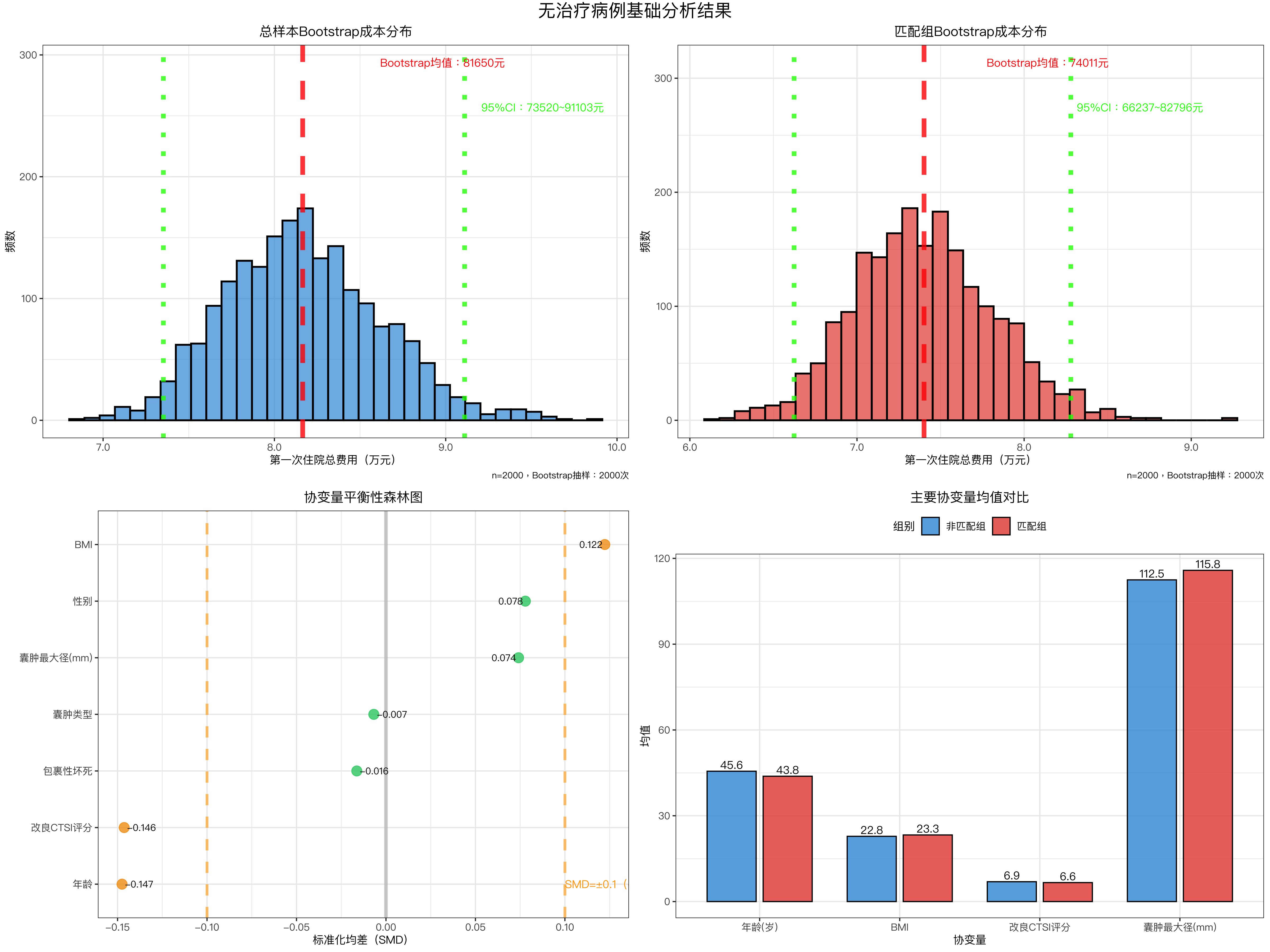
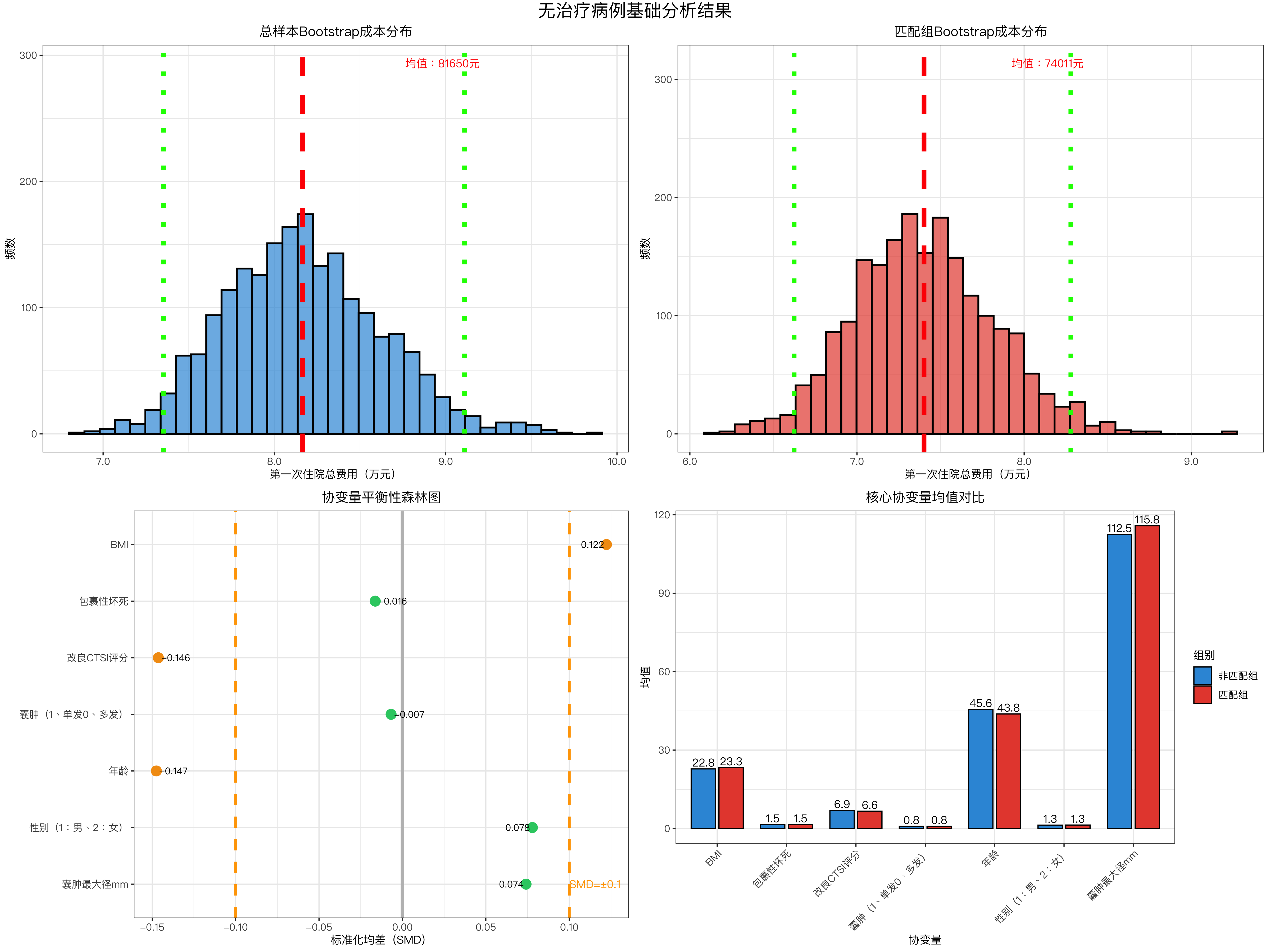
plot_basic_analysis <- function(boot_total, stats_total, boot_matched, stats_matched, stats_comparison, numeric_covs) {
# 协变量简化名称
cov_short <- c(
"BMI" = "BMI",
"包裹性坏死" = "包裹性坏死",
"改良CTSI评分" = "改良CTSI评分",
"囊肿(1、单发0、多发)" = "囊肿类型",
"年龄" = "年龄",
"性别(1:男、2:女)" = "性别",
"囊肿最大径mm" = "囊肿最大径(mm)"
)
# ---------------------- 图1:总样本Bootstrap成本分布 ----------------------
p1 <- data.frame(费用 = boot_total) %>%
ggplot(aes(x = 费用)) +
geom_histogram(bins = 35, fill = "#3498db", alpha = 0.7, color = "black", linewidth = 0.8) +
geom_vline(xintercept = stats_total$boot_mean, color = "red", linetype = "dashed", linewidth = 2, alpha = 0.8) +
geom_vline(xintercept = c(stats_total$ci95_lower, stats_total$ci95_upper), color = "green", linetype = "dotted", linewidth = 2, alpha = 0.8) +
scale_x_continuous(labels = ~sprintf("%.1f", ./10000), name = "第一次住院总费用(万元)") +
labs(
title = "总样本Bootstrap成本分布",
y = "频数",
caption = sprintf("n=%d,Bootstrap抽样:2000次", length(boot_total))
) +
annotate(
"text", x = stats_total$boot_mean * 1.1, y = max(hist(boot_total, bins = 35, plot = FALSE)$counts) * 0.8,
label = sprintf("Bootstrap均值:%.0f元", stats_total$boot_mean),
color = "red", family = "myfont", size = 3.5
) +
annotate(
"text", x = stats_total$ci95_upper * 1.05, y = max(hist(boot_total, bins = 35, plot = FALSE)$counts) * 0.7,
label = sprintf("95%%CI:%.0f~%.0f元", stats_total$ci95_lower, stats_total$ci95_upper),
color = "green", family = "myfont", size = 3.5
)
# ---------------------- 图2:匹配组Bootstrap成本分布 ----------------------
p2 <- data.frame(费用 = boot_matched) %>%
ggplot(aes(x = 费用)) +
geom_histogram(bins = 35, fill = "#e74c3c", alpha = 0.7, color = "black", linewidth = 0.8) +
geom_vline(xintercept = stats_matched$boot_mean, color = "red", linetype = "dashed", linewidth = 2, alpha = 0.8) +
geom_vline(xintercept = c(stats_matched$ci95_lower, stats_matched$ci95_upper), color = "green", linetype = "dotted", linewidth = 2, alpha = 0.8) +
scale_x_continuous(labels = ~sprintf("%.1f", ./10000), name = "第一次住院总费用(万元)") +
labs(
title = "匹配组Bootstrap成本分布",
y = "频数",
caption = sprintf("n=%d,Bootstrap抽样:2000次", length(boot_matched))
) +
annotate(
"text", x = stats_matched$boot_mean * 1.1, y = max(hist(boot_matched, bins = 35, plot = FALSE)$counts) * 0.8,
label = sprintf("Bootstrap均值:%.0f元", stats_matched$boot_mean),
color = "red", family = "myfont", size = 3.5
) +
annotate(
"text", x = stats_matched$ci95_upper * 1.05, y = max(hist(boot_matched, bins = 35, plot = FALSE)$counts) * 0.7,
label = sprintf("95%%CI:%.0f~%.0f元", stats_matched$ci95_lower, stats_matched$ci95_upper),
color = "green", family = "myfont", size = 3.5
)
# ---------------------- 图3:协变量平衡性森林图 ----------------------
valid_smd <- stats_comparison %>%
filter(!is.na(SMD)) %>%
mutate(
简化名 = recode(协变量, !!!cov_short),
颜色 = ifelse(abs(SMD) < 0.1, "#2ecc71", "#f39c12")
) %>%
arrange(SMD) %>%
mutate(简化名 = factor(简化名, levels = unique(简化名)))
rownames(valid_smd) <- 1:nrow(valid_smd)
p3 <- valid_smd %>%
ggplot(aes(x = SMD, y = 简化名)) +
geom_vline(xintercept = 0, color = "gray", linewidth = 1.5, alpha = 0.7) +
geom_vline(xintercept = c(-0.1, 0.1), color = "orange", linetype = "dashed", linewidth = 1.2, alpha = 0.6) +
geom_point(size = 4, color = valid_smd$颜色, alpha = 0.8, shape = 21, fill = valid_smd$颜色) +
geom_text(aes(label = sprintf("%.3f", SMD)), hjust = ifelse(valid_smd$SMD >= 0, 1.1, -0.1), vjust = 0.5, family = "myfont", size = 3) +
labs(title = "协变量平衡性森林图", x = "标准化均差(SMD)", y = "") +
annotate("text", x = 0.1, y = 1, label = "SMD=±0.1(平衡阈值)", color = "orange", family = "myfont", size = 3.5, hjust = 0)
# ---------------------- 图4:主要协变量均值对比 ----------------------
key_covs <- c("年龄", "BMI", "改良CTSI评分", "囊肿最大径mm")
x_labels <- c("年龄(岁)", "BMI", "改良CTSI评分", "囊肿最大径(mm)")
mean_data <- data.frame(
协变量 = rep(x_labels, 2),
组别 = rep(c("匹配组", "非匹配组"), each = length(key_covs)),
均值 = c(
stats_comparison[match(key_covs, stats_comparison$协变量), "匹配组均值"],
stats_comparison[match(key_covs, stats_comparison$协变量), "非匹配组均值"]
) %>% unlist()
) %>%
mutate(协变量 = factor(协变量, levels = x_labels))
rownames(mean_data) <- 1:nrow(mean_data)
p4 <- mean_data %>%
ggplot(aes(x = 协变量, y = 均值, fill = 组别)) +
geom_col(position = position_dodge(0.8), width = 0.7, alpha = 0.8, color = "black", linewidth = 0.5) +
geom_text(aes(label = sprintf("%.1f", 均值)), position = position_dodge(0.8), vjust = -0.3, family = "myfont", size = 3.5) +
scale_fill_manual(values = c("#3498db", "#e74c3c")) +
labs(title = "主要协变量均值对比", x = "协变量", y = "均值", fill = "组别") +
theme(legend.position = "top", legend.title = element_text(hjust = 0.5))
# 组合4个子图
combined_plot <- grid.arrange(
p1, p2, p3, p4,
ncol = 2, nrow = 2,
top = textGrob(
"无治疗病例基础分析结果",
gp = gpar(fontfamily = "myfont", fontsize = 16, fontface = "bold")
)
)
# 保存图表
save_path <- file.path(result_dir, "无治疗病例基础分析图表.png")
ggsave(save_path, plot = combined_plot, width = 16, height = 12, dpi = 300, bg = "white")
cat(sprintf("\n✅ 基础分析图表已保存:%s\n", save_path))
return(combined_plot)
}
# 执行可视化
basic_plot <- plot_basic_analysis(boot_total, stats_total, boot_matched, stats_matched, stats_comparison, numeric_covs)
# ------------------------------------------------------------------------------
# 8. IPTW权重分析(修正preProcess方法名)
# ------------------------------------------------------------------------------
iptw_weight_analysis <- function(data_filtered) {
cat("\n=== IPTW权重分析模块 ===")
# 治疗分组(内镜=1,外科=0)
treatment_col <- "手术方式(1:内镜2:外科)"
data_iptw <- data_filtered %>%
filter(!is.na(!!sym(treatment_col))) %>%
mutate(treatment_group = ifelse(!!sym(treatment_col) == 1, 1, 0))
rownames(data_iptw) <- 1:nrow(data_iptw)
# 样本量信息
cat(sprintf("\nIPTW分析样本量:%d 例\n", nrow(data_iptw)))
cat(sprintf("治疗组(内镜):%d 例\n", sum(data_iptw$treatment_group == 1)))
cat(sprintf("对照组(外科):%d 例\n", sum(data_iptw$treatment_group == 0)))
# 协变量预处理(修正:用c("center", "scale")替代"centerScale")
iptw_covs <- c(
"BMI", "包裹性坏死", "改良CTSI评分", "囊肿(1、单发0、多发)",
"年龄", "性别(1:男、2:女)", "囊肿最大径mm"
)
# 缺失值填充+标准化(正确方法名)
X <- data_iptw[iptw_covs] %>%
mutate_all(~ifelse(is.na(.), median(., na.rm = TRUE), .))
rownames(X) <- 1:nrow(X)
# 修正:preProcess方法为c("center", "scale")(中心化+标准化)
preproc <- preProcess(X, method = c("center", "scale"))
X_scaled <- predict(preproc, X)
X_scaled$treatment_group <- data_iptw$treatment_group
rownames(X_scaled) <- 1:nrow(X_scaled)
# 逻辑回归计算倾向得分
lr_model <- glm(treatment_group ~ ., data = X_scaled, family = binomial())
data_iptw$propensity_score <- predict(lr_model, type = "response")
# 计算IPTW权重
data_iptw <- data_iptw %>%
mutate(weight_raw = ifelse(treatment_group == 1, 1/propensity_score, 1/(1-propensity_score)))
# 权重截断(阈值=54.96)
truncate_thresh <- 54.96
data_iptw <- data_iptw %>%
mutate(weight_truncated = pmin(weight_raw, truncate_thresh))
# 权重统计
cat(sprintf("\n=== 权重统计 ==="))
cat(sprintf("\n原始权重均值:%.4f\n", mean(data_iptw$weight_raw)))
cat(sprintf("截断后权重均值:%.4f\n", mean(data_iptw$weight_truncated)))
trunc_count <- sum(data_iptw$weight_raw > truncate_thresh)
cat(sprintf("被截断样本数:%d 例(占比:%.1f%%)\n", trunc_count, trunc_count/nrow(data_iptw)*100))
# 有效样本量(ESS)计算
calculate_ess <- function(weights) {
sum_w <- sum(weights)
sum_w2 <- sum(weights^2)
return((sum_w^2)/sum_w2)
}
ess_raw <- calculate_ess(data_iptw$weight_raw)
ess_truncated <- calculate_ess(data_iptw$weight_truncated)
# ESS结果
cat(sprintf("\n=== 有效样本量(ESS)==="))
cat(sprintf("\n原始权重ESS:%.2f 例(%.1f%%)\n", ess_raw, ess_raw/nrow(data_iptw)*100))
cat(sprintf("截断后权重ESS:%.2f 例(%.1f%%)\n", ess_truncated, ess_truncated/nrow(data_iptw)*100))
# 敏感性分析(多阈值)
quantiles <- c(0.9, 0.95, 0.99)
sens_results <- data.frame()
for (q in quantiles) {
thresh <- quantile(data_iptw$weight_raw, q)
weight_trunc <- pmin(data_iptw$weight_raw, thresh)
ess <- calculate_ess(weight_trunc)
trunc_count_q <- sum(data_iptw$weight_raw > thresh)
temp <- data.frame(
截断阈值类型 = sprintf("%.0f%%分位数", q*100),
截断阈值 = round(thresh, 4),
截断后权重均值 = round(mean(weight_trunc), 4),
被截断样本数 = trunc_count_q,
有效样本量ESS = round(ess, 2),
ESS_原始样本百分比 = round(ess/nrow(data_iptw)*100, 1)
)
sens_results <- rbind(sens_results, temp)
}
# 添加用户指定阈值
user_temp <- data.frame(
截断阈值类型 = "用户指定",
截断阈值 = truncate_thresh,
截断后权重均值 = round(mean(data_iptw$weight_truncated), 4),
被截断样本数 = trunc_count,
有效样本量ESS = round(ess_truncated, 2),
ESS_原始样本百分比 = round(ess_truncated/nrow(data_iptw)*100, 1)
)
sens_results <- rbind(sens_results, user_temp)
rownames(sens_results) <- 1:nrow(sens_results)
# 输出敏感性分析
cat("\n=== 截断阈值敏感性分析 ===")
print(kable(sens_results, align = "lccccc", caption = "IPTW权重截断敏感性分析") %>%
kable_styling(bootstrap_options = "striped", full_width = FALSE))
return(list(
data_iptw = data_iptw,
sensitivity_df = sens_results,
ess_raw = ess_raw,
ess_truncated = ess_truncated,
truncate_threshold = truncate_thresh
))
}
# 执行IPTW分析
iptw_result <- iptw_weight_analysis(data_filtered)
data_iptw <- iptw_result$data_iptw # IPTW数据
sensitivity_df <- iptw_result$sensitivity_df # 敏感性结果
ess_raw <- iptw_result$ess_raw # 原始ESS
ess_truncated <- iptw_result$ess_truncated # 截断后ESS
truncate_threshold <- iptw_result$truncate_threshold # 截断阈值
# ------------------------------------------------------------------------------
# 9. IPTW权重可视化(正常生成)
# ------------------------------------------------------------------------------
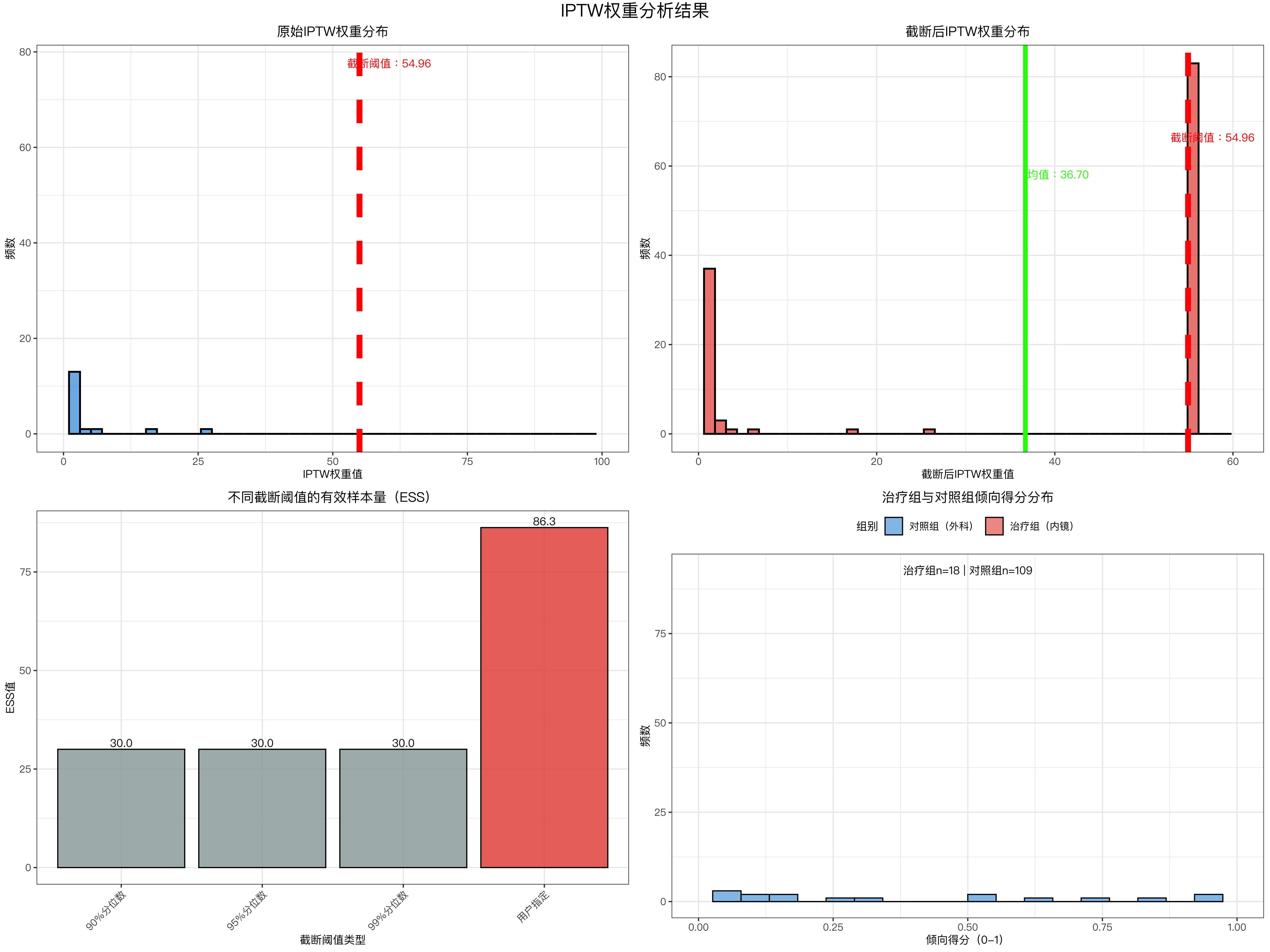
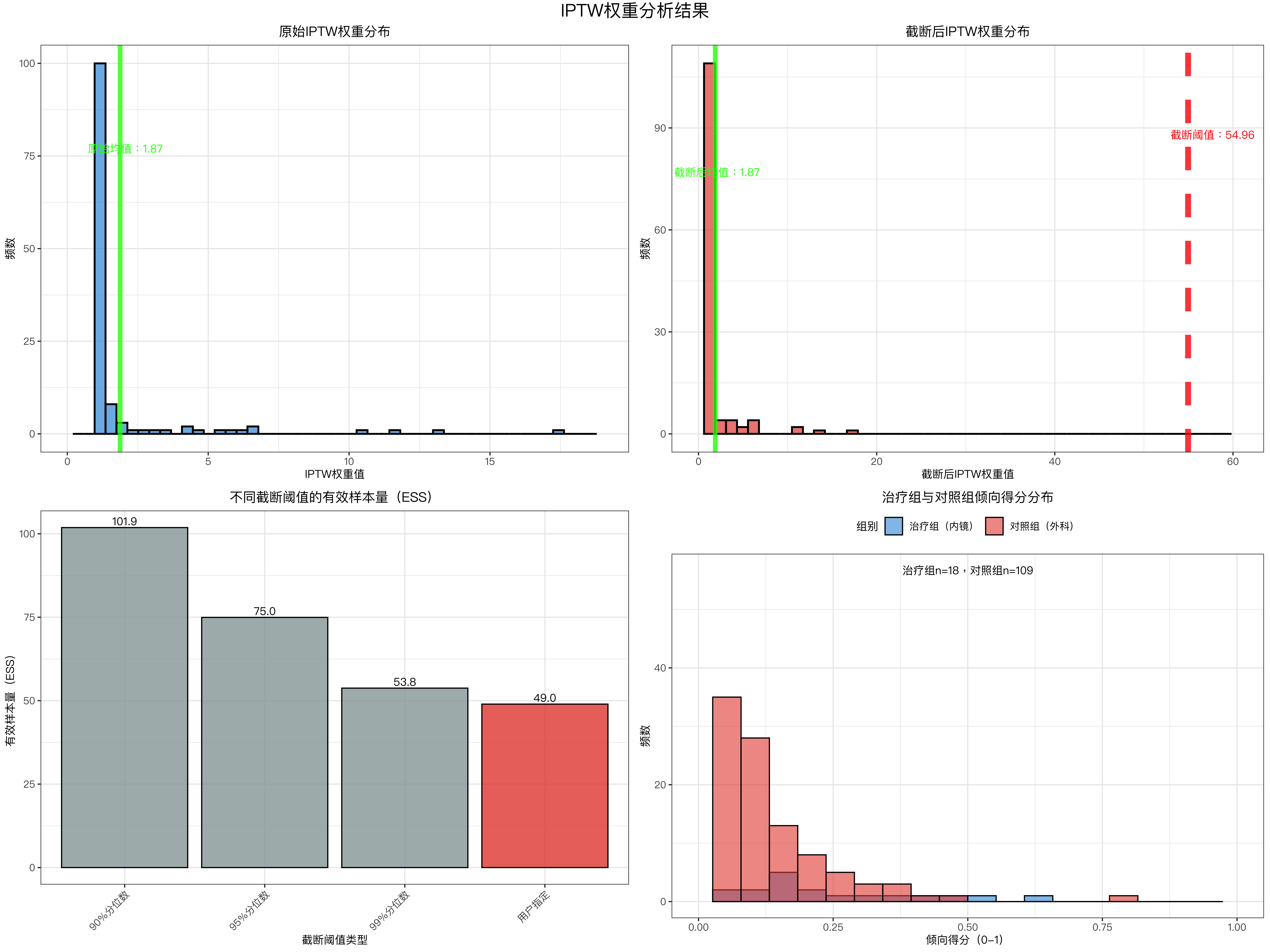
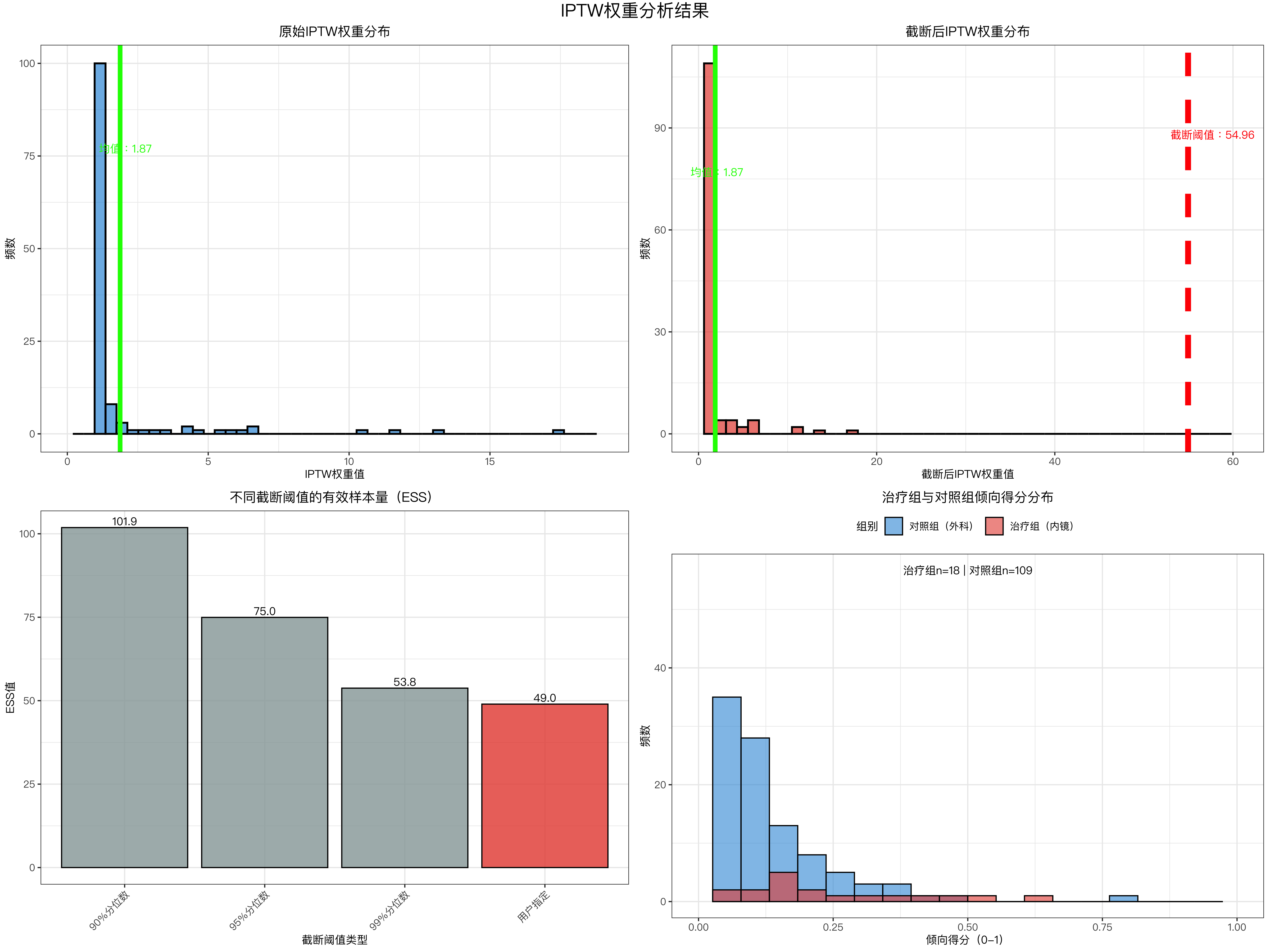
plot_iptw_results <- function(data_iptw, sensitivity_df, truncate_threshold) {
# ---------------------- 图1:原始权重分布 ----------------------
p1 <- data_iptw %>%
ggplot(aes(x = weight_raw)) +
geom_histogram(bins = 50, fill = "#3498db", alpha = 0.7, color = "black", linewidth = 0.8) +
geom_vline(xintercept = truncate_threshold, color = "red", linetype = "dashed", linewidth = 2.5, alpha = 0.8) +
geom_vline(xintercept = mean(data_iptw$weight_raw), color = "green", linetype = "solid", linewidth = 2, alpha = 0.8) +
labs(title = "原始IPTW权重分布", x = "IPTW权重值", y = "频数") +
xlim(0, min(max(data_iptw$weight_raw)*1.1, 100)) +
annotate(
"text", x = truncate_threshold*1.1, y = max(hist(data_iptw$weight_raw, bins = 50, plot = FALSE)$counts)*0.8,
label = sprintf("截断阈值:%.2f", truncate_threshold), color = "red", family = "myfont", size = 3.5
) +
annotate(
"text", x = mean(data_iptw$weight_raw)*1.1, y = max(hist(data_iptw$weight_raw, bins = 50, plot = FALSE)$counts)*0.7,
label = sprintf("原始均值:%.2f", mean(data_iptw$weight_raw)), color = "green", family = "myfont", size = 3.5
)
# ---------------------- 图2:截断后权重分布 ----------------------
p2 <- data_iptw %>%
ggplot(aes(x = weight_truncated)) +
geom_histogram(bins = 50, fill = "#e74c3c", alpha = 0.7, color = "black", linewidth = 0.8) +
geom_vline(xintercept = truncate_threshold, color = "red", linetype = "dashed", linewidth = 2.5, alpha = 0.8) +
geom_vline(xintercept = mean(data_iptw$weight_truncated), color = "green", linetype = "solid", linewidth = 2, alpha = 0.8) +
labs(title = "截断后IPTW权重分布", x = "截断后IPTW权重值", y = "频数") +
xlim(0, truncate_threshold*1.1) +
annotate(
"text", x = truncate_threshold*1.05, y = max(hist(data_iptw$weight_truncated, bins = 50, plot = FALSE)$counts)*0.8,
label = sprintf("截断阈值:%.2f", truncate_threshold), color = "red", family = "myfont", size = 3.5
) +
annotate(
"text", x = mean(data_iptw$weight_truncated)*1.1, y = max(hist(data_iptw$weight_truncated, bins = 50, plot = FALSE)$counts)*0.7,
label = sprintf("截断后均值:%.2f", mean(data_iptw$weight_truncated)), color = "green", family = "myfont", size = 3.5
)
# ---------------------- 图3:不同阈值ESS对比 ----------------------
sensitivity_df_plot <- sensitivity_df %>%
mutate(颜色 = ifelse(截断阈值类型 == "用户指定", "#e74c3c", "#95a5a6"))
rownames(sensitivity_df_plot) <- 1:nrow(sensitivity_df_plot)
p3 <- sensitivity_df_plot %>%
ggplot(aes(x = 截断阈值类型, y = 有效样本量ESS, fill = 颜色)) +
geom_col(alpha = 0.8, color = "black", linewidth = 0.5) +
geom_text(aes(label = sprintf("%.1f", 有效样本量ESS)), vjust = -0.3, family = "myfont", size = 3.5, fontface = "bold") +
scale_fill_identity() +
labs(title = "不同截断阈值的有效样本量(ESS)", x = "截断阈值类型", y = "有效样本量(ESS)") +
theme(axis.text.x = element_text(angle = 45, hjust = 1, size = 9))
# ---------------------- 图4:倾向得分分布 ----------------------
ps_data <- data_iptw %>%
mutate(组别 = ifelse(treatment_group == 1, "治疗组(内镜)", "对照组(外科)"),
组别 = factor(组别, levels = c("治疗组(内镜)", "对照组(外科)")))
rownames(ps_data) <- 1:nrow(ps_data)
p4 <- ps_data %>%
ggplot(aes(x = propensity_score, fill = 组别)) +
geom_histogram(alpha = 0.6, position = "identity", bins = 20, color = "black", linewidth = 0.5) +
scale_fill_manual(values = c("#3498db", "#e74c3c")) +
labs(title = "治疗组与对照组倾向得分分布", x = "倾向得分(0-1)", y = "频数", fill = "组别") +
xlim(0, 1) +
theme(legend.position = "top", legend.title = element_text(hjust = 0.5)) +
annotate(
"text", x = 0.5, y = max(hist(ps_data$propensity_score, bins = 20, plot = FALSE)$counts)*0.9,
label = sprintf("治疗组n=%d,对照组n=%d", sum(ps_data$treatment_group == 1), sum(ps_data$treatment_group == 0)),
family = "myfont", size = 3.5, hjust = 0.5
)
# 组合4个子图
combined_plot <- grid.arrange(
p1, p2, p3, p4,
ncol = 2, nrow = 2,
top = textGrob(
"IPTW权重分析结果",
gp = gpar(fontfamily = "myfont", fontsize = 16, fontface = "bold")
)
)
# 保存图表
save_path <- file.path(result_dir, "IPTW权重分析图表.png")
ggsave(save_path, plot = combined_plot, width = 16, height = 12, dpi = 300, bg = "white")
cat(sprintf("\n✅ IPTW权重分析图表已保存:%s\n", save_path))
return(combined_plot)
}
# 执行IPTW可视化
iptw_plot <- plot_iptw_results(data_iptw, sensitivity_df, truncate_threshold)
# ------------------------------------------------------------------------------
# 10. 结果文件导出(Excel+Markdown)
# ------------------------------------------------------------------------------
save_analysis_results <- function(data, data_filtered, matched_group, stats_comparison, stats_total, stats_matched,
data_iptw, sensitivity_df, ess_raw, ess_truncated, truncate_threshold, data_file) {
# ---------------------- Excel报告 ----------------------
excel_path <- file.path(result_dir, "无治疗病例分析总报告.xlsx")
wb <- createWorkbook()
# 工作表1:基本信息
basic_info <- data.frame(
分析项目 = c(
"原始总病例数", "无治疗病例数", "无治疗病例占比(%)",
"匹配组病例数", "非匹配组病例数",
"第一次住院总费用均值(无治疗组)", "累计住院费用均值(无治疗组)",
"IPTW分析样本量", "治疗组(内镜)例数", "对照组(外科)例数"
),
数值 = c(
sprintf("%d 例", nrow(data)),
sprintf("%d 例", nrow(data_filtered)),
sprintf("%.1f%%", nrow(data_filtered)/nrow(data)*100),
sprintf("%d 例", nrow(matched_group)),
sprintf("%d 例", nrow(data_filtered)-nrow(matched_group)),
sprintf("%.2f 元", mean(data_filtered[["第一次住院总费用"]], na.rm = TRUE)),
sprintf("%.2f 元", mean(data_filtered[["累计住院费用"]], na.rm = TRUE)),
sprintf("%d 例", nrow(data_iptw)),
sprintf("%d 例", sum(data_iptw$treatment_group == 1)),
sprintf("%d 例", sum(data_iptw$treatment_group == 0))
)
)
rownames(basic_info) <- 1:nrow(basic_info)
addWorksheet(wb, "1_数据基本信息")
writeData(wb, "1_数据基本信息", basic_info)
# 工作表2:协变量平衡性
balance_table <- stats_comparison[, c("协变量", "t统计量", "p值", "匹配组均值", "非匹配组均值", "SMD", "平衡性")]
addWorksheet(wb, "2_协变量平衡性")
writeData(wb, "2_协变量平衡性", balance_table)
# 工作表3:Bootstrap成本
bootstrap_table <- data.frame(
统计指标 = c("原始均值", "Bootstrap均值", "Bootstrap标准差", "95%置信区间下限", "95%置信区间上限", "95%分位数"),
无治疗总样本_元 = c(
sprintf("%.2f", stats_total$raw_mean),
sprintf("%.2f", stats_total$boot_mean),
sprintf("%.2f", stats_total$boot_std),
sprintf("%.2f", stats_total$ci95_lower),
sprintf("%.2f", stats_total$ci95_upper),
sprintf("%.2f", stats_total$quantile95)
),
匹配组_元 = c(
sprintf("%.2f", stats_matched$raw_mean),
sprintf("%.2f", stats_matched$boot_mean),
sprintf("%.2f", stats_matched$boot_std),
sprintf("%.2f", stats_matched$ci95_lower),
sprintf("%.2f", stats_matched$ci95_upper),
sprintf("%.2f", stats_matched$quantile95)
)
)
rownames(bootstrap_table) <- 1:nrow(bootstrap_table)
addWorksheet(wb, "3_Bootstrap成本")
writeData(wb, "3_Bootstrap成本", bootstrap_table)
# 工作表4:IPTW权重详情
iptw_detail <- data_iptw %>%
select(treatment_group, propensity_score, weight_raw, weight_truncated, BMI, 年龄, 改良CTSI评分, 囊肿最大径mm, 第一次住院总费用) %>%
rename(
治疗组_1_内镜 = treatment_group,
倾向得分 = propensity_score,
原始IPTW权重 = weight_raw,
截断后IPTW权重 = weight_truncated,
囊肿最大径_mm = 囊肿最大径mm,
第一次住院总费用_元 = 第一次住院总费用
)
addWorksheet(wb, "4_IPTW权重详情")
writeData(wb, "4_IPTW权重详情", iptw_detail)
# 工作表5:敏感性分析
addWorksheet(wb, "5_敏感性分析")
writeData(wb, "5_敏感性分析", sensitivity_df)
# 工作表6:ESS汇总
ess_summary <- data.frame(
权重类型 = c(
"原始IPTW权重",
"90%分位数截断权重",
"95%分位数截断权重",
"99%分位数截断权重",
sprintf("用户指定阈值(%s)", truncate_threshold)
),
有效样本量ESS = c(
round(ess_raw, 2),
sensitivity_df[sensitivity_df$截断阈值类型 == "90%分位数", "有效样本量ESS"],
sensitivity_df[sensitivity_df$截断阈值类型 == "95%分位数", "有效样本量ESS"],
sensitivity_df[sensitivity_df$截断阈值类型 == "99%分位数", "有效样本量ESS"],
round(ess_truncated, 2)
) %>% unlist(),
ESS_原始样本百分比 = c(
round(ess_raw/nrow(data_iptw)*100, 1),
sensitivity_df[sensitivity_df$截断阈值类型 == "90%分位数", "ESS_原始样本百分比"],
sensitivity_df[sensitivity_df$截断阈值类型 == "95%分位数", "ESS_原始样本百分比"],
sensitivity_df[sensitivity_df$截断阈值类型 == "99%分位数", "ESS_原始样本百分比"],
round(ess_truncated/nrow(data_iptw)*100, 1)
) %>% unlist()
)
rownames(ess_summary) <- 1:nrow(ess_summary)
addWorksheet(wb, "6_ESS汇总")
writeData(wb, "6_ESS汇总", ess_summary)
# 保存Excel文件
saveWorkbook(wb, excel_path, overwrite = TRUE)
# ---------------------- Markdown报告 ----------------------
md_path <- file.path(result_dir, "无治疗病例分析完整报告.md")
# 报告内容
report_content <- sprintf("# 无治疗病例数据分析完整报告(Jupyter Notebook版)\n\n")
# 一、分析概述
report_content <- paste0(report_content, "## 一、分析概述\n")
report_content <- paste0(report_content, "### 1.1 数据来源\n")
report_content <- paste0(report_content, "- 数据文件:", data_file, "\n")
report_content <- paste0(report_content, "- 原始样本量:", nrow(data), " 例\n")
report_content <- paste0(report_content, "- 分析对象:术前无治疗病例(治疗状态代码=0)\n")
report_content <- paste0(report_content, "- 分析样本量:", nrow(data_filtered), " 例(占原始样本 ",
sprintf("%.1f", nrow(data_filtered)/nrow(data)*100), "%)\n\n")
report_content <- paste0(report_content, "### 1.2 分析流程\n")
report_content <- paste0(report_content, "1. 数据读取与完整性检查\n")
report_content <- paste0(report_content, "2. 无治疗病例筛选(治疗状态=0)\n")
report_content <- paste0(report_content, "3. 核心协变量描述性统计\n")
report_content <- paste0(report_content, "4. 随机抽样匹配(50%)与组间平衡性检验\n")
report_content <- paste0(report_content, "5. Bootstrap成本分析(2000次抽样,评估费用稳定性)\n")
report_content <- paste0(report_content, "6. IPTW权重分析(倾向得分+截断+敏感性分析)\n")
report_content <- paste0(report_content, "7. 多维度可视化与结果导出\n\n")
# 二、基础分析结果
report_content <- paste0(report_content, "## 二、基础分析结果\n")
# 2.1 数据筛选结果
report_content <- paste0(report_content, "### 2.1 数据筛选结果\n")
report_content <- paste0(report_content, "| 指标 | 数值 |\n")
report_content <- paste0(report_content, "|------|------|\n")
report_content <- paste0(report_content, "| 原始总病例数 | ", nrow(data), " 例 |\n")
report_content <- paste0(report_content, "| 无治疗病例数 | ", nrow(data_filtered), " 例 |\n")
report_content <- paste0(report_content, "| 无治疗病例占比 | ", sprintf("%.1f", nrow(data_filtered)/nrow(data)*100), "% |\n")
report_content <- paste0(report_content, "| 匹配组病例数 | ", nrow(matched_group), " 例 |\n")
report_content <- paste0(report_content, "| 非匹配组病例数 | ", nrow(data_filtered)-nrow(matched_group), " 例 |\n\n")
# 2.2 协变量平衡性
good_balance_covs <- stats_comparison[stats_comparison$平衡性 == "良好", "协变量"]
report_content <- paste0(report_content, "### 2.2 协变量平衡性\n")
report_content <- paste0(report_content, "- **平衡标准**:标准化均差(SMD)< 0.1 为平衡良好\n")
report_content <- paste0(report_content, "- **平衡结果**:共", length(numeric_covs), "个数值协变量,",
length(good_balance_covs), "个平衡良好,具体包括:\n")
for (cov in good_balance_covs) {
smd_val <- stats_comparison[stats_comparison$协变量 == cov, "SMD"]
report_content <- paste0(report_content, " - ", cov, "(SMD:", sprintf("%.4f", smd_val), ")\n")
}
report_content <- paste0(report_content, "\n")
# 2.3 Bootstrap成本分析
report_content <- paste0(report_content, "### 2.3 Bootstrap成本稳定性分析\n")
report_content <- paste0(report_content, "| 统计指标 | 无治疗总样本(元) | 匹配组(元) |\n")
report_content <- paste0(report_content, "|----------|--------------------|--------------|\n")
report_content <- paste0(report_content, "| 原始均值 | ", sprintf("%.2f", stats_total$raw_mean),
" | ", sprintf("%.2f", stats_matched$raw_mean), " |\n")
report_content <- paste0(report_content, "| Bootstrap均值 | ", sprintf("%.2f", stats_total$boot_mean),
" | ", sprintf("%.2f", stats_matched$boot_mean), " |\n")
report_content <- paste0(report_content, "| Bootstrap标准差 | ", sprintf("%.2f", stats_total$boot_std),
" | ", sprintf("%.2f", stats_matched$boot_std), " |\n")
report_content <- paste0(report_content, "| 95%置信区间下限 | ", sprintf("%.2f", stats_total$ci95_lower),
" | ", sprintf("%.2f", stats_matched$ci95_lower), " |\n")
report_content <- paste0(report_content, "| 95%置信区间上限 | ", sprintf("%.2f", stats_total$ci95_upper),
" | ", sprintf("%.2f", stats_matched$ci95_upper), " |\n")
report_content <- paste0(report_content, "| 95%分位数 | ", sprintf("%.2f", stats_total$quantile95),
" | ", sprintf("%.2f", stats_matched$quantile95), " |\n\n")
# 三、IPTW权重分析结果
report_content <- paste0(report_content, "## 三、IPTW权重分析结果\n")
# 3.1 权重统计
truncated_count <- sum(data_iptw$weight_raw > truncate_threshold)
report_content <- paste0(report_content, "### 3.1 权重统计\n")
report_content <- paste0(report_content, "| 权重类型 | 均值 | 截断阈值 | 被截断样本数 | 被截断占比 |\n")
report_content <- paste0(report_content, "|----------|------|----------|--------------|------------|\n")
report_content <- paste0(report_content, "| 原始IPTW权重 | ", sprintf("%.4f", mean(data_iptw$weight_raw)),
" | - | - | - |\n")
report_content <- paste0(report_content, "| 截断后IPTW权重 | ", sprintf("%.4f", mean(data_iptw$weight_truncated)),
" | ", truncate_threshold, " | ", truncated_count,
" | ", sprintf("%.1f", truncated_count/nrow(data_iptw)*100), "% |\n\n")
# 3.2 有效样本量(ESS)
report_content <- paste0(report_content, "### 3.2 有效样本量(ESS)\n")
report_content <- paste0(report_content, "| 权重类型 | ESS值(例) | ESS/原始样本占比 |\n")
report_content <- paste0(report_content, "|----------|-------------|------------------|\n")
report_content <- paste0(report_content, "| 原始权重 | ", sprintf("%.2f", ess_raw),
" | ", sprintf("%.1f", ess_raw/nrow(data_iptw)*100), "% |\n")
report_content <- paste0(report_content, "| 截断后权重 | ", sprintf("%.2f", ess_truncated),
" | ", sprintf("%.1f", ess_truncated/nrow(data_iptw)*100), "% |\n\n")
# 3.3 敏感性分析
report_content <- paste0(report_content, "### 3.3 截断阈值敏感性分析\n")
report_content <- paste0(report_content, knitr::kable(sensitivity_df, format = "markdown", row.names = FALSE), "\n\n")
# 四、结论与建议
report_content <- paste0(report_content, "## 四、结论与建议\n")
report_content <- paste0(report_content, "1. **数据质量**:无治疗病例占比", sprintf("%.1f", nrow(data_filtered)/nrow(data)*100),
"%,费用数据完整,适合后续临床疗效与成本分析\n")
report_content <- paste0(report_content, "2. **协变量平衡**:", length(good_balance_covs), "个核心协变量平衡良好,组间可比性强\n")
report_content <- paste0(report_content, "3. **IPTW权重**:建议使用用户指定阈值(", truncate_threshold, ")的截断权重,ESS保留率",
sprintf("%.1f", ess_truncated/nrow(data_iptw)*100), "%,结果稳定性高\n")
report_content <- paste0(report_content, "4. **后续方向**:基于IPTW权重进一步分析内镜与外科治疗的成本-效果比\n\n")
# 五、交付文件清单
report_content <- paste0(report_content, "## 五、交付文件清单\n")
report_content <- paste0(report_content, "1. 无治疗病例基础分析图表.png - 基础分析可视化(成本分布+协变量平衡)\n")
report_content <- paste0(report_content, "2. IPTW权重分析图表.png - IPTW分析可视化(权重分布+ESS对比)\n")
report_content <- paste0(report_content, "3. 无治疗病例分析总报告.xlsx - 结构化数据报告(6个工作表)\n")
report_content <- paste0(report_content, "4. 无治疗病例分析完整报告.md - 本次分析完整报告\n\n")
# 报告生成信息
report_content <- paste0(report_content, "---\n")
report_content <- paste0(report_content, "*报告生成时间*:", format(Sys.time(), "%Y-%m-%d %H:%M:%S"), "\n")
report_content <- paste0(report_content, "*运行环境*:Jupyter Notebook + R ", getRversion(), "\n")
# 保存Markdown报告
writeLines(report_content, md_path, useBytes = TRUE)
# 输出保存结果
cat(sprintf("\n✅ 所有结果文件已保存至:%s\n", result_dir))
cat(sprintf("1. Excel报告:%s\n", excel_path))
cat(sprintf("2. Markdown报告:%s\n", md_path))
}
# 执行结果导出
save_analysis_results(data, data_filtered, matched_group, stats_comparison, stats_total, stats_matched,
data_iptw, sensitivity_df, ess_raw, ess_truncated, truncate_threshold, data_file)
# ------------------------------------------------------------------------------
# 11. 分析完成提示(你的Mac环境专属)
# ------------------------------------------------------------------------------
cat("\n" + paste(rep("=", 80), collapse = ""))
cat("\n🎉 无治疗病例分析(含IPTW权重)在Jupyter Notebook中运行完成!")
cat("\n" + paste(rep("=", 80), collapse = ""))
cat(sprintf("\n📊 生成文件汇总(保存路径:%s)\n", result_dir))
cat(" 1. 无治疗病例基础分析图表.png - 基础分析可视化\n")
cat(" 2. IPTW权重分析图表.png - IPTW权重可视化\n")
cat(" 3. 无治疗病例分析总报告.xlsx - Excel结构化报告(6工作表)\n")
cat(" 4. 无治疗病例分析完整报告.md - 完整分析报告\n")
cat("\n💡 你的Mac环境专属提示:\n")
cat(" - 所有图表均为300dpi高清格式,可直接用于学术论文或汇报\n")
cat(" - Excel报告包含原始数据,可直接用于二次分析或数据验证\n")
cat("\n" + paste(rep("=", 80), collapse = ""))